7 data visualization techniques that every data scientist should know
by Claudia Boker
In the ever-expanding world of data science, the ability to effectively communicate insights is a skill that sets apart exceptional data scientists.
As data volumes continue to grow exponentially, the need to transform complex datasets into visually compelling narratives becomes increasingly critical. This is where data visualization emerges as an indispensable tool. By harnessing the power of visual representation, data scientists can distill complicated information into easy-to-understand visualizations that are relatable to audiences and facilitate informed decision-making.
This blog post will delve into seven essential data visualization techniques that every data scientist should master. These techniques include:
Through a detailed exploration of these seven techniques, this blog post aims to equip data scientists with the knowledge and skills necessary to leverage the full potential of data visualization. The post will provide:
• use cases
• discuss how to create and interpret graphs and charts
• tips for enhancing the effectiveness of the visualization
Whether you are presenting findings to stakeholders, collaborating with colleagues, or influencing decision-makers, mastering these techniques will enable you to communicate complex ideas with clarity, impact, and persuasion.
Join us as we unveil the power of data visualization! By the end of this blog post, you will have the tools and expertise needed to transform raw data into captivating visual narratives that inform, inspire, and drive meaningful action. Get ready to become a master storyteller with data!
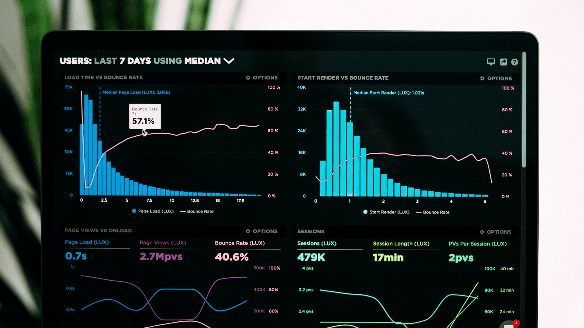
A bar chart, also known as a bar graph, is a visual representation of data that utilizes rectangular bars with varying heights or lengths. The length or height of each bar in a bar chart represents how many times or how much of something is associated with a specific category. The taller the bar, the larger the value or frequency it represents for that category.

Bar charts are a helpful tool for understanding data by visually showing patterns and relationships. They are great for comparing data across categories. In a bar chart, the rectangular bars have different lengths, and the height or length of each bar shows the magnitude or frequency of the data. This makes it simple to spot patterns, trends, and differences between categories. Whether you're examining sales, survey results, or population numbers, bar charts provide a clear and easy-to-understand way to share information. They are essential for analyzing and effectively communicating data.
“Bar charts often compare categories, but that’s not always the case. You just need a discrete variable for the horizontal X-axis…Assess the differences between bars to evaluate how the metric changes between discrete values. Identify the groups that have the highest and lowest values. ”
Longer or taller bars indicate larger values. Look for patterns, trends, or disparities across different categories. Compare the heights of the bars to identify higher or lower values. The spacing between bars represents the distinction between categories.

Line graphs are commonly used to analyze and present time-series data, such as stock market trends, weather patterns, or population growth over time. Additionally, line graphs can be employed to track changes in metrics like sales figures, website traffic, or social media engagement. They are especially useful for illustrating trends, patterns, or changes in data over time, making them a valuable tool for displaying temporal information.
By visualizing the data on a line graph, you can uncover insights, detect anomalies, and make predictions based on the observed patterns and trends.
A scatter plot is a graphical representation that shows the relationship between two numerical variables. It utilizes dots to represent data points, with each dot representing the values of the two variables being compared. By examining a scatter plot, we can identify patterns or connections between the variables. It helps us understand how the variables change together and if there are any outliers or distinctive groups of data points. In simpler terms, a scatter plot helps us visualize and comprehend the relationship between two sets of numbers.

Scatter plots are valuable tools used in practical scenarios. For instance, they can illustrate how house prices change based on the size of the house. In education, scatter plots help us understand if studying more hours leads to higher exam scores. In business, they facilitate the analysis of the link between advertising spending and sales revenue. For retailers, scatter plots can showcase how temperature affects ice cream sales. In human resources, scatter plots can unveil connections between employee experience and salary. These examples demonstrate how scatter plots assist in comprehending relationships between different factors in a straightforward manner.
By following these steps and considering the context of the data, you can gain valuable insights from a scatter plot and interpret the relationship between the variables it represents.

By incorporating these tips, you can create scatter plots that effectively display relationships, convey information clearly, and capture viewers' attention.


Both correlation and categorical heatmaps are useful for analyzing data and uncovering patterns, but they are used with several types of variables. Correlation heatmaps are applicable to numerical values, while categorical heatmaps work with categories or groups. The choice depends on the type of data and the specific questions you aim to address.
Intensity or density heatmaps find applications in various domains, including website analytics, risk assessment, population density analysis, disease outbreak tracking, weather forecasting, and sports analysis. On the other hand, correlation heatmaps are useful in feature selection, data exploration, multivariate analysis, trends analysis, and anomaly detection. They help identify important variables, understand relationships, uncover complex associations, detect temporal trends, and identify outliers. Categorical heatmaps find utility in market research, genetics and bioinformatics, social sciences, data clustering, and performance evaluation. They assist in analyzing consumer preferences, visualizing gene expression patterns, studying survey responses, identifying clusters, and evaluating performance across categories. Both correlation and categorical heatmaps provide valuable insights across various domains, enabling pattern recognition, data exploration, and decision-making.
Remember that interpreting heat maps is subjective and context-dependent. Consider the context and your understanding of the data. Considering the data being shown and any background information will aid in interpreting the heatmap accurately.
1. Choose clear colors: Select colors that accurately represent the data and are easily interpretable. Use distinguishable colors that intuitively convey the information. Avoid color schemes that might cause confusion or misinterpretation.
2. Strategically order and group variables: Arrange variables in a way that improves the readability and interpretability of the heatmap. For correlation heatmaps, consider grouping highly correlated variables together to reveal patterns and clusters more effectively. In categorical heatmaps, order categories logically based on frequency or a meaningful sequence for your data.
3. Add informative annotations: Enhance the interpretation of your heatmap by including labels, titles, or explanatory notes. These additional annotations provide context and clarify the representation of the heatmap. They assist viewers in understanding the data and any relevant details associated with it.
By incorporating these suggestions, you can enhance the quality of your heatmaps, making them clearer, more accurate, and easier to interpret.
Box plots, also known as box-and-whisker plots, are simple graphical representations that show the distribution of a set of data. They provide a summary of the data's center, spread, and shape. A box plot displays five main statistics: the smallest value, the lower quartile (25th percentile), the median (50th percentile), the upper quartile (75th percentile), and the largest value. Additionally, box spots may show lines, called whiskers, which extend to the smallest and largest values, as well as any exceptional values, known as outliers.

Box plots have practical uses in various scenarios. They are valuable for exploring data and quickly understanding how data is spread out when comparing multiple groups or categories. They assist in identifying outliers, which are values that significantly differ from the rest. Box plots facilitate comparisons of distributions between different datasets or groups, enabling the observation of variations in center, spread, and variability. They are widely used for statistical analysis to assess differences between groups and are effective in presenting statistical information in reports, research papers, or presentations, enhancing clarity and highlighting important insights.
Remember, interpreting box and whisker plots provides an overview of the data's distribution, including measures of central tendency, variability, and the presence of outliers. It helps you gain insights into the dataset without needing to examine each value.
By following these tips, you can make your box plots easier to understand, visually appealing, and more effective in communicating information to your audience. Let’s look at the last data visualization technique.

The primary purpose of a violin plot is to display the distribution of data and compare it across multiple categories or groups. It offers a way to visualize the shape, spread, and multimodality of the data, allowing for insights into the underlying patterns and variations. Violin plots are particularly useful when dealing with complex datasets with many categories or when comparing multiple distributions simultaneously.
Violin plots have several practical use cases. They can be used for comparing distributions of a continuous variable across different groups, such as comparing blood pressure levels between patients who received different treatments in a medical study. Violin plots are also helpful in visualizing demographic characteristics, like comparing income levels among various education levels or age groups. Also ideal for analyzing time series data, revealing seasonal patterns or trends. In evaluating performance, violin plots can assess the distribution of prediction errors across different models, providing insights for improvement. Additionally, during data exploration, violin plots quickly convey the distribution of a variable, including skewness, multimodality, and outliers.
Interactive visualizations have various applications across different fields. They are useful for data exploration, enabling users to navigate through complex datasets and discover hidden insights. In business intelligence, interactive visualizations help users analyze performance metrics and make informed decisions. In data journalism, readers can interact with visualization to explore different aspects and understand the underlying story. Additionally, interactive visualizations facilitate collaborative data analysis, allowing teams to work together and collectively analyze and interpret data. Overall, interactive visualizations empower users to actively interact with data, promoting a deeper understanding and enhancing decision-making processes.
These tools offer different levels of customization, ease of use, and compatibility with programming languages. Choosing the right tool depends on factors such as data complexity, desired interactivity, and collaboration needs.


Both Matplotlib and Seaborn are extensively documented and have active user communities, making it easier to find examples, tutorials, and support when working with these libraries. They are widely adopted in the Python ecosystem and offer compatibility with other libraries and frameworks, making them suitable for various visualization needs.
By leveraging the styling capabilities of Matplotlib and Seaborn, you can apply consistent and visually appealing styles to all types of visualizations, regardless of the technique you choose. Whether you are creating basic line charts, bar plots, scatter plots, or advanced statistical visualizations, these libraries empower you to customize and enhance the appearance of your Python visualizations to effectively communicate your data and insights.
It is important for data scientists to continually explore and learn new visualization techniques. The field of data visualization is always evolving, with new tools and approaches emerging regularly. By staying curious and adaptable, data scientists can leverage these advancements to create more impactful and innovative visualizations.
Styling plays a significant role in data visualization using Python. Python offers libraries like Matplotlib, Seaborn, and Plotly, which provide extensive styling options to customize visual elements such as colors, fonts, labels, and axes. By applying appropriate styling techniques, data scientists can enhance the visual appeal of their plots, improve readability, and reinforce their intended message.
To summarize, mastering data visualization involves understanding essential techniques, selecting the appropriate visualization method, continuously exploring new techniques, and utilizing styling options in Python. By following these practices, data scientists can effectively communicate complex information, engage their audience, and drive informed decision-making.
If this article has piqued your interest in learning more about data science and data science techniques, we encourage you to check out our Data Science bootcamp. Our bootcamp provides comprehensive training and practical hands-on experience in data science, including data visualization, statistical analysis, machine learning, and more. To learn more about our Data Science bootcamp, please visit https://learning.constructor.org/data-science/zurich. Start your journey toward becoming a proficient data scientist today!
As data volumes continue to grow exponentially, the need to transform complex datasets into visually compelling narratives becomes increasingly critical. This is where data visualization emerges as an indispensable tool. By harnessing the power of visual representation, data scientists can distill complicated information into easy-to-understand visualizations that are relatable to audiences and facilitate informed decision-making.
This blog post will delve into seven essential data visualization techniques that every data scientist should master. These techniques include:
- bar charts
- line graphs
- scatter plots
- heatmaps
- box plots
- violin plots
- interactive visualizations
Through a detailed exploration of these seven techniques, this blog post aims to equip data scientists with the knowledge and skills necessary to leverage the full potential of data visualization. The post will provide:
• use cases
• discuss how to create and interpret graphs and charts
• tips for enhancing the effectiveness of the visualization
Whether you are presenting findings to stakeholders, collaborating with colleagues, or influencing decision-makers, mastering these techniques will enable you to communicate complex ideas with clarity, impact, and persuasion.
Join us as we unveil the power of data visualization! By the end of this blog post, you will have the tools and expertise needed to transform raw data into captivating visual narratives that inform, inspire, and drive meaningful action. Get ready to become a master storyteller with data!
Bar charts
A bar chart, also known as a bar graph, is a visual representation of data that utilizes rectangular bars with varying heights or lengths. The length or height of each bar in a bar chart represents how many times or how much of something is associated with a specific category. The taller the bar, the larger the value or frequency it represents for that category.Bar charts are a helpful tool for understanding data by visually showing patterns and relationships. They are great for comparing data across categories. In a bar chart, the rectangular bars have different lengths, and the height or length of each bar shows the magnitude or frequency of the data. This makes it simple to spot patterns, trends, and differences between categories. Whether you're examining sales, survey results, or population numbers, bar charts provide a clear and easy-to-understand way to share information. They are essential for analyzing and effectively communicating data.
Interpreting bar charts:
Interpreting a bar chart involves analyzing the heights or lengths of the bars and making comparisons between categories. As Jim explains in his article “Bar Charts: Using, Examples, and Interpreting”:“Bar charts often compare categories, but that’s not always the case. You just need a discrete variable for the horizontal X-axis…Assess the differences between bars to evaluate how the metric changes between discrete values. Identify the groups that have the highest and lowest values. ”
Longer or taller bars indicate larger values. Look for patterns, trends, or disparities across different categories. Compare the heights of the bars to identify higher or lower values. The spacing between bars represents the distinction between categories.
Here are some simple tips to make your bar charts better:
- Arrange bars in a logical order: Organize the bars in a logical order that facilitates easy comparison and understanding of the data. This could involve arranging them in ascending or descending order, chronological order, or any other relevant order based on the nature of the data.
- Utilize buckets: Buckets help simplify complex data sets and make it easier to interpret the information presented in the chart. Grouping and summarizing data using buckets provides a clearer overview or comparison of different categories or ranges. By employing buckets, you can effectively highlight patterns, trends, or distributions within the data.
- Ensure proper scaling: Pay attention to the scaling of your bar chart to accurately represent the data. Avoid distorting the visual representation by using inappropriate scales that can mislead viewers.
- Select the appropriate type of bar chart: There are various types of bar charts, such as vertical bar charts (column charts) and horizontal bar charts (bar graphs). Choose the type that best fits your data and the message you want to convey. Horizontal bar charts are particularly useful when dealing with lengthy headers as they allow for easy horizontal reading without the need to turn one's head vertically.
Line graph
Line graphs are graphical representations that use lines to connect data points. According to Chartio, a line chart is a graphical representation that highlights changes in values for one variable (plotted on the vertical axis) over a continuous range of a second variable (plotted on the horizontal axis).Line graphs are commonly used to analyze and present time-series data, such as stock market trends, weather patterns, or population growth over time. Additionally, line graphs can be employed to track changes in metrics like sales figures, website traffic, or social media engagement. They are especially useful for illustrating trends, patterns, or changes in data over time, making them a valuable tool for displaying temporal information.
Interpreting line graphs:
To better understand a line graph and derive insights from the data, follow these steps:- Examine slope and direction: Analyze the slopes of the lines to identify increasing, decreasing, or constant trends.
- Identify patterns: Look for consistent trends, fluctuations, or cycles in the overall shape of the graph.
- Evaluate the rate of change: Consider the steepness of the lines to understand the speed of change.
- Note intersections and overlaps: Identify where lines intersect or overlap to observe relationships between variables.
- Consider outliers and anomalies: Take note of data points that deviate significantly from the overall pattern and investigate their significance.
By visualizing the data on a line graph, you can uncover insights, detect anomalies, and make predictions based on the observed patterns and trends.
Here are some simple tips to make your line graphs better:
- Zero-value baseline: As Mike Yi writes, unlike bar charts and histograms, line charts don’t necessarily require a zero baseline on the vertical axis. The focus of a line chart is to show changes in value rather than the absolute values themselves. Therefore, it's acceptable to adjust the vertical axis range in line charts to highlight meaningful changes in value without adhering strictly to a zero baseline.
- Simplify and declutter: Keep your line graph clean and uncluttered by removing any unnecessary elements. Avoid excessive gridlines, decorations, or annotations that may distract viewers from the main data trends. Strive for simplicity to ensure that the key information stands out prominently.
- Limit the number of lines: If you have too many lines, consider reducing the number of variables or categories you are representing. Focusing on the most important or relevant data points will prevent overcrowding the graph and make te graph easier to interpret. Selecting a subset of lines that best convey your message can enhance clarity and avoid overwhelming the viewer.
Scatter Plots
A scatter plot is a graphical representation that shows the relationship between two numerical variables. It utilizes dots to represent data points, with each dot representing the values of the two variables being compared. By examining a scatter plot, we can identify patterns or connections between the variables. It helps us understand how the variables change together and if there are any outliers or distinctive groups of data points. In simpler terms, a scatter plot helps us visualize and comprehend the relationship between two sets of numbers.Scatter plots are valuable tools used in practical scenarios. For instance, they can illustrate how house prices change based on the size of the house. In education, scatter plots help us understand if studying more hours leads to higher exam scores. In business, they facilitate the analysis of the link between advertising spending and sales revenue. For retailers, scatter plots can showcase how temperature affects ice cream sales. In human resources, scatter plots can unveil connections between employee experience and salary. These examples demonstrate how scatter plots assist in comprehending relationships between different factors in a straightforward manner.
Interpreting scatter plots:
Interpreting a scatter plot involves understanding the relationship between two variables and identifying any patterns, trends, or correlations that may exist. Here's a step-by-step guide on how to effectively interpret a scatter plot:- Examine the data distribution: Look at the overall distribution of the data points. Are they concentrated in a particular region, or are they spread out? This initial observation can provide insights into the pattern or lack thereof in the data.
- Determine the direction of the relationship: Examine the movement of the data points. If they generally move from the bottom left to the top right, it indicates a positive relationship - meaning that as one variable increases, the other tends to increase as well. Conversely, if the data points move from the top left to the bottom right, it suggests a negative relationship. If no discernible pattern exists, it may indicate no relationship or a weak correlation.
- Identify the strength of the relationship: Consider how closely the data points cluster around a line or curve. If they are tightly clustered and form a distinct line or curve, it suggests a strong relationship. On the other hand, if the points are more scattered and don't follow a specific pattern, it indicates a weak relationship or no correlation.
- Assess the correlation: To quantify the relationship between variables, calculate the correlation coefficient. This value ranges from -1 to 1. A value near 1 or -1 signifies a strong positive or negative correlation, while a value near 0 indicates a weak or no correlation.
By following these steps and considering the context of the data, you can gain valuable insights from a scatter plot and interpret the relationship between the variables it represents.
Here are some simple tips to make your scatter plots better:
Now that we've covered the basics of interpreting a scatter plot, let's explore some simple tips to enhance the effectiveness of your scatter plot.- Data point transparency: If there are many overlapping data points, utilize transparency or alpha blending to visually emphasize the density of the data.
- Consistent data representation: Ensure that the data points are consistently plotted throughout the scatter plot. Use the same symbol, size, and color for all data points to maintain consistency. However, you can introduce variations in these attributes to represent different variables or categories between the datasets. By doing so, you can convey multiple dimensions of information.
- Avoid overplotting: Overplotting occurs when multiple data points are plotted in such a way that they overlap, making it difficult to discern individual points or patterns. To mitigate overplotting, consider techniques such as jittering, alpha blending, or reducing the size of data points.
- Add a trendline: As mentioned by Mike Yi in his article: “A Complete Guide to Scatter Plots”, incorporating a trendline in a scatter plot can be a useful technique to visualize and highlight the overall relationship or trend between the variables. It can provide insights into the general direction and strength of the correlation.
By incorporating these tips, you can create scatter plots that effectively display relationships, convey information clearly, and capture viewers' attention.
Heatmaps
There are different types of heatmaps, such as example intensity or density heatmaps, which graphically represent data using colors to depict varying levels of intensity or density. They are commonly used to display data on a two-dimensional surface, like a map or a grid, where each data point is assigned, a color based on its value. In this discussion, we will focus on correlation and categorical heatmaps.1. Correlation heatmap:
A correlation heatmap shows the relationships between different numbers in a dataset. It utilizes colors to represent the strength and direction of these relationships. Colors ranging from red to blue indicate positive and negative correlations, respectively. Correlation heatmaps are useful for identifying patterns and connections among numerical values.
2. Categorical heatmap:
A categorical heatmap helps us understand the relationships between various categories or groups within a dataset. It employs colors to display the frequency or count of observations within each category combination. Categorical heat maps are valuable for identifying patterns and distributions within various groups.Both correlation and categorical heatmaps are useful for analyzing data and uncovering patterns, but they are used with several types of variables. Correlation heatmaps are applicable to numerical values, while categorical heatmaps work with categories or groups. The choice depends on the type of data and the specific questions you aim to address.
Intensity or density heatmaps find applications in various domains, including website analytics, risk assessment, population density analysis, disease outbreak tracking, weather forecasting, and sports analysis. On the other hand, correlation heatmaps are useful in feature selection, data exploration, multivariate analysis, trends analysis, and anomaly detection. They help identify important variables, understand relationships, uncover complex associations, detect temporal trends, and identify outliers. Categorical heatmaps find utility in market research, genetics and bioinformatics, social sciences, data clustering, and performance evaluation. They assist in analyzing consumer preferences, visualizing gene expression patterns, studying survey responses, identifying clusters, and evaluating performance across categories. Both correlation and categorical heatmaps provide valuable insights across various domains, enabling pattern recognition, data exploration, and decision-making.
Interpreting heatmaps:
Interpreting heatmaps involves understanding the colors and the data they represent. Here are some guidelines to help with the interpretation:Correlation heatmaps:
- Color representation: warmer colors (e.g. red) typically indicate positive correlations, while cooler colors (e.g. blue) indicate negative correlations. The intensity of the color represents the strength of the correlation.
- Pattern identification: Look for clusters or groups of variables with similar color patterns, indicating strong correlations.
- Correlation values: Some heatmaps may display the actual correlation values within each cell. Pay attention to high values (close to 1 or -1) as they indicate a strong relationship between the corresponding variables.
Categorical heatmaps:
- Color representation: Colors represent the frequency or count of observations within each category combination. The intensity or shade of the color may reflect the magnitude of the count or frequency.
- Pattern identification: Look for areas of high or low intensity in the heatmap, indicating categories or combinations that have a higher or lower frequency of observations.
- Comparisons: Compare the color intensities between different rows or columns to identify differences in frequency or count across categories or groups.
Remember that interpreting heat maps is subjective and context-dependent. Consider the context and your understanding of the data. Considering the data being shown and any background information will aid in interpreting the heatmap accurately.
Here are some simple tips to make your heatmaps better:
To enhance the effectiveness and clarity of your heatmaps, consider the following strategies:1. Choose clear colors: Select colors that accurately represent the data and are easily interpretable. Use distinguishable colors that intuitively convey the information. Avoid color schemes that might cause confusion or misinterpretation.
2. Strategically order and group variables: Arrange variables in a way that improves the readability and interpretability of the heatmap. For correlation heatmaps, consider grouping highly correlated variables together to reveal patterns and clusters more effectively. In categorical heatmaps, order categories logically based on frequency or a meaningful sequence for your data.
3. Add informative annotations: Enhance the interpretation of your heatmap by including labels, titles, or explanatory notes. These additional annotations provide context and clarify the representation of the heatmap. They assist viewers in understanding the data and any relevant details associated with it.
By incorporating these suggestions, you can enhance the quality of your heatmaps, making them clearer, more accurate, and easier to interpret.
Box plots
Box plots, also known as box-and-whisker plots, are simple graphical representations that show the distribution of a set of data. They provide a summary of the data's center, spread, and shape. A box plot displays five main statistics: the smallest value, the lower quartile (25th percentile), the median (50th percentile), the upper quartile (75th percentile), and the largest value. Additionally, box spots may show lines, called whiskers, which extend to the smallest and largest values, as well as any exceptional values, known as outliers.Box plots have practical uses in various scenarios. They are valuable for exploring data and quickly understanding how data is spread out when comparing multiple groups or categories. They assist in identifying outliers, which are values that significantly differ from the rest. Box plots facilitate comparisons of distributions between different datasets or groups, enabling the observation of variations in center, spread, and variability. They are widely used for statistical analysis to assess differences between groups and are effective in presenting statistical information in reports, research papers, or presentations, enhancing clarity and highlighting important insights.
Interpreting box plots:
Interpreting box plots and whisker plots involves examining the key elements of the plot to understand the distribution of the data. Here's a step-by-step guide:- Identify the median: The line inside the box represents the median, which is the middle value of the dataset. It divides the data into two halves.
- Determine the quartiles: The box is drawn from the first quartile (Q1) to the upper quartile (Q3). Q1 represents the 25th percentile, indicating the point below which 25% of the data falls. Q3 represents the 75th percentile, below which 75% of the data falls.
- Check the spread: The length of the box called the interquartile range (IQR), shows the range where the middle 50% of the data lies. It is calculated as IQR = Q3 - Q1.
- Examine the whiskers: The lines extending from the box indicate the range of the data, excluding outliers. They reach up to the minimum and maximum values within a specified range.
- Spot outliers: Outliers are values that fall far outside the whiskers. They are shown as individual points or asterisks. Outliers can represent exceptional or unusual values that significantly differ from the rest of the data.
- Consider symmetry and skewness: Look at the position of the median within the box and the lengths of the whiskers. If the whiskers are similar in length and the median is in the middle of the box, the distribution is likely symmetric. Skewness may be present if one whisker is noticeably longer.
- Compare multiple box plots: If you have multiple box plots, compare the position and shape of the boxes and whiskers. This allows you to understand differences in center, spread, and variability across diverse groups or categories.
Remember, interpreting box and whisker plots provides an overview of the data's distribution, including measures of central tendency, variability, and the presence of outliers. It helps you gain insights into the dataset without needing to examine each value.
Here are some simple tips to make your box plots better:
To enhance the effectiveness and visual appeal of your box plots, consider the following tips:- Clear labeling and context: Make sure to label the axes and provide a title that explains what the box plot represents. If you are comparing different groups or categories, use a legend or color-coded labels to show the differences. Adding explanatory notes can also help viewers understand the meaning of the data and the insights being presented.
- Consistent scale and axis range: Keep the scale and range of the axes consistent across multiple box plots or when comparing different variables. This means using the same measurement units and ensuring the axes cover the entire range of the data. Consistency helps viewers accurately interpret the positions, spreads, and variations within the box plots.
By following these tips, you can make your box plots easier to understand, visually appealing, and more effective in communicating information to your audience. Let’s look at the last data visualization technique.
Violin plots
A violin plot is a type of data visualization that combines features of a box plot and a kernel density plot. It provides a concise summary of the distribution of a continuous variable across different categories or groups. The plot resembles a violin, with a thickened body in the middle representing the bulk of the data and thinner sections, known as "hinges," on either side indicating the less frequent values.The primary purpose of a violin plot is to display the distribution of data and compare it across multiple categories or groups. It offers a way to visualize the shape, spread, and multimodality of the data, allowing for insights into the underlying patterns and variations. Violin plots are particularly useful when dealing with complex datasets with many categories or when comparing multiple distributions simultaneously.
Violin plots have several practical use cases. They can be used for comparing distributions of a continuous variable across different groups, such as comparing blood pressure levels between patients who received different treatments in a medical study. Violin plots are also helpful in visualizing demographic characteristics, like comparing income levels among various education levels or age groups. Also ideal for analyzing time series data, revealing seasonal patterns or trends. In evaluating performance, violin plots can assess the distribution of prediction errors across different models, providing insights for improvement. Additionally, during data exploration, violin plots quickly convey the distribution of a variable, including skewness, multimodality, and outliers.
Interpreting violin plots:
Violin plots are captivating visualizations that can provide valuable insights into your data. If you're new to this type of plot, fear not! Here is a simple four-step guide to help you interpret violin plots like a pro.- Identify the shape and spread: Take a moment to observe the violin plot's overall shape. Imagine it as an actual violin – the wider parts represent areas with more data points, while the narrower sections suggest fewer points. Keep an eye out for any interesting features like asymmetry, peaks, or gaps, as they can reveal intriguing patterns within your data.
- Compare violin plots: If you have multiple violin plots in one visualization, it's time to compare them. Look for differences in width, height, or the presence of multiple peaks. By doing so, you can uncover variations in the distributions across different groups or categories. Maybe one group has a broader spread, or perhaps you notice a significant difference in density. Comparisons bring out valuable insights.
- Examine the hinges and tails: Now, focus your attention on the hinges – those little marks on the sides of the violin. They represent the lower and upper quartiles of your data. Are they at the same height, or does one extend higher than the other? Additionally, take note of the tails, which stretch beyond the hinges. Tails can indicate the presence of outliers or unusual data points that don't conform to the main distribution. Understanding these aspects helps you grasp the central tendencies, spread, and potential outliers in your data.
- Consider additional information: Violin plots often come with other elements, such as box plots or point markers. Don't overlook them! Box plots provide valuable details about the median, quartiles, and potential outliers. Point markers, on the other hand, indicate individual data points and offer a glimpse into the granularity of your data. By considering these additional components, you gain a more comprehensive understanding of the distribution and any noteworthy characteristics present.
Here are some simple tips to make your violin plots better:
Here are two tips to keep in mind when making your next violin plot.- Make it visually appealing: Customize the appearance of your violin plot to make it visually appealing and easy to understand. You can choose different colors for each group or category to make them stand out. Also, consider adjusting the thickness of the lines or making them more transparent to improve clarity. Experiment with different styles until you find the one that looks best and helps convey your data effectively. Just remember not to overcomplicate it or sacrifice readability.
- Add helpful labels: Use labels to provide additional information and make your violin plot more informative. You can label specific data points or outliers that are worth noting. Additionally, consider adding text or arrows to highlight important patterns or trends in the plot. Labeling makes it easier for your audience to understand the key insights without getting overwhelmed. However, be careful not to add too many labels, as it can clutter the plot and confuse viewers.
Interactive visualizations
These are dynamic representations of data that allow users to actively engage with the information. Unlike static visualizations, interactive visualizations let users manipulate and explore the data in real-time. They have features like zooming, filtering, and sorting, which users can interact with to customize the visualization. By actively engaging with the visualization, users can uncover patterns, relationships, and trends that may not be apparent in static visuals. This interactive approach encourages exploration and helps users gain valuable insights through an intuitive and engaging interface.Interactive visualizations have various applications across different fields. They are useful for data exploration, enabling users to navigate through complex datasets and discover hidden insights. In business intelligence, interactive visualizations help users analyze performance metrics and make informed decisions. In data journalism, readers can interact with visualization to explore different aspects and understand the underlying story. Additionally, interactive visualizations facilitate collaborative data analysis, allowing teams to work together and collectively analyze and interpret data. Overall, interactive visualizations empower users to actively interact with data, promoting a deeper understanding and enhancing decision-making processes.
Tools and technologies for creating interactive visualizations
Interactive visualizations have become increasingly popular due to their ability to engage users and provide more immersive data experiences. As data-driven decision-making becomes more prevalent across industries, the demand for tools and technologies that enable interactive visualizations has grown. Here are some popular tools and technologies used for creating interactive visualizations:- D3.js: A powerful JavaScript library for creating customizable visualizations using HTML, CSS, and SVG elements.
- Tableau: An intuitive data visualization tool with a drag-and-drop interface, ideal for creating interactive dashboards and reports.
- Power BI: A Microsoft tool for business analytics, allowing for the creation of interactive visualizations, real-time updates, and collaboration.
- Plotly: A versatile JavaScript library supporting Python, R, and JavaScript, offering a wide range of interactive chart types and animation options.
- Tableau Public: A free web-based platform for creating and sharing interactive visualizations publicly, suitable for data storytelling.
- ggplot2: An R package for creating interactive visualizations using the grammar of graphics, providing a concise and consistent syntax.
- Highcharts: A JavaScript charting library offering interactive features like tooltips, zooming, and panning, with various chart types available.
These tools offer different levels of customization, ease of use, and compatibility with programming languages. Choosing the right tool depends on factors such as data complexity, desired interactivity, and collaboration needs.
Tips for designing engaging and interactive visualizations
Designing engaging and interactive visualizations requires careful consideration. Here are some tips to elevate the impact of your visualizations:- Choose the right chart type: Select the appropriate chart that suits your data and message.
- Keep it simple: Avoid clutter and focus on the essential information. Use clear labels and eliminate unnecessary elements.
- Use color strategically: Employ a consistent color scheme to highlight important aspects of your data.
- Incorporate interactivity: Add interactive elements like tooltips and filters to engage users.
- Provide context and storytelling: Guide viewers through your visualization with annotations and narratives.
- Optimize for different devices: Ensure your visualizations are responsive across various devices.
- Test and iterate: Gather feedback and refine your visualizations for continuous improvement.
Bonus tips
Logarithmic scales
- What is this you might ask, logarithmic scales are commonly used on charts to represent data that spans a wide range of magnitudes or values. Here are a few situations where logarithmic scales are particularly useful:
- Wide range of values: When your data spans a large range of magnitudes, logarithmic scales can help present the data effectively. They prevent smaller values from being overshadowed by larger ones, making it easier to visualize the entire range.
- Exponential growth or decay: If your data exhibits exponential growth or decay, logarithmic scales can highlight the rate of change. This is especially useful for data related to population growth, economic trends, or the spread of a virus.
- Relative changes: Logarithmic scales are effective for comparing relative changes between values rather than absolute differences. They are commonly used in stock market analysis to compare the performance of different stocks over time.
- Financial data: Logarithmic scales are commonly used in financial charts, such as stock prices or market indices. Since financial data often involves large fluctuations, logarithmic scales can help identify long-term trends while still showing smaller changes.
- Scientific and engineering data: Logarithmic scales are popular in scientific and engineering fields when dealing with measurements that span multiple orders of magnitude. Examples include seismic activity, sound intensity, pH levels, and signal strength.
Controlling styling in Python
When you control the styling in Python, you can make your visualizations look better and match your brand or design preferences. With libraries like Matplotlib or Seaborn, you can adjust things like the font, color, lines, and markers in your visualizations. By changing these settings, you can create visuals that have the look you want and show your message clearly. Trying out different styles and exploring the options helps you make your Python visualizations look polished and professional. Regardless of the visualization technique you choose, these libraries offer extensive styling capabilities to enhance the visual appeal and clarity of your visualizations.- Matplotlib is a versatile plotting library that provides a wide range of functions for creating different types of visualizations. It allows you to control the styling of elements such as axes, grids, labels, titles, and legends. Matplotlib offers flexibility in customizing line styles, marker types, colors, and other visual properties to create visually appealing plots. It is a foundational library widely used in scientific, engineering, and data analysis domains.
- Seaborn, on the other hand, is a higher-level library built on top of Matplotlib. It offers a more streamlined interface and provides additional statistical plotting capabilities. Seaborn simplifies the process of creating complex visualizations such as statistical models, regression plots, heatmaps, and categorical plots. It also comes with built-in color palettes and style templates, making it easier to create visually pleasing and consistent visualizations.
Both Matplotlib and Seaborn are extensively documented and have active user communities, making it easier to find examples, tutorials, and support when working with these libraries. They are widely adopted in the Python ecosystem and offer compatibility with other libraries and frameworks, making them suitable for various visualization needs.
By leveraging the styling capabilities of Matplotlib and Seaborn, you can apply consistent and visually appealing styles to all types of visualizations, regardless of the technique you choose. Whether you are creating basic line charts, bar plots, scatter plots, or advanced statistical visualizations, these libraries empower you to customize and enhance the appearance of your Python visualizations to effectively communicate your data and insights.
Conclusion
In conclusion, we have covered five essential data visualization techniques: bar charts, line charts, scatter plots, heatmaps, interactive charts, box plots, and violin plots. Each technique has its own advantages and is suitable for different types of data and analysis purposes. Choosing the right visualization technique is crucial because it ensures clear and visually appealing representations of data, allowing viewers to quickly understand patterns and relationships.It is important for data scientists to continually explore and learn new visualization techniques. The field of data visualization is always evolving, with new tools and approaches emerging regularly. By staying curious and adaptable, data scientists can leverage these advancements to create more impactful and innovative visualizations.
Styling plays a significant role in data visualization using Python. Python offers libraries like Matplotlib, Seaborn, and Plotly, which provide extensive styling options to customize visual elements such as colors, fonts, labels, and axes. By applying appropriate styling techniques, data scientists can enhance the visual appeal of their plots, improve readability, and reinforce their intended message.
To summarize, mastering data visualization involves understanding essential techniques, selecting the appropriate visualization method, continuously exploring new techniques, and utilizing styling options in Python. By following these practices, data scientists can effectively communicate complex information, engage their audience, and drive informed decision-making.
If this article has piqued your interest in learning more about data science and data science techniques, we encourage you to check out our Data Science bootcamp. Our bootcamp provides comprehensive training and practical hands-on experience in data science, including data visualization, statistical analysis, machine learning, and more. To learn more about our Data Science bootcamp, please visit https://learning.constructor.org/data-science/zurich. Start your journey toward becoming a proficient data scientist today!